Line profiles are everywhere in microscopy. You draw a line across a structure, measure the full width at half maximum, and call it your resolution. It is quick, it is visual, and it is one of the most biased things you can do to a good image.
I want to make the case for retiring the line profile as a resolution metric — not as a display tool, which it is fine for, but as the number you report when someone asks how well your microscope resolves. And I want to point you to what I use instead.
Why the line profile misleads you
The problem is not the maths. The full width at half maximum of a well-sampled cross-section is a perfectly reasonable quantity. The problem is everything you decide before you compute it.
You pick where to draw the line. In practice that means you drift toward the sharpest-looking cross-section in the field, because that is the one that looks convincing. You also need a thin, isolated, well-oriented structure to measure across — so the method silently excludes the parts of the image where resolution is actually being tested. And the number you walk away with comes from one location in one image, maybe a handful if you do a little statistics.
That number tells you how sharp that one structure looks. It does not tell you the resolution of your image. Those are different claims, and the gap between them is exactly where selection bias lives.
A line profile answers "how narrow is this feature?" The question you usually mean to ask is "at what spatial frequency does my image stop carrying real information?" The second question is about the whole image, and it does not let you cherry-pick the measurement site.
A parameter-free alternative: decorrelation analysis
The method I recommend is the decorrelation analysis published by Adrien Descloux, Kristin Grußmayer and Aleksandra Radenovic in Nature Methods in 2019. Its central virtue is that it extracts a resolution estimate from a single image with no user-defined parameters — nothing to draw, nothing to orient, nothing to choose.
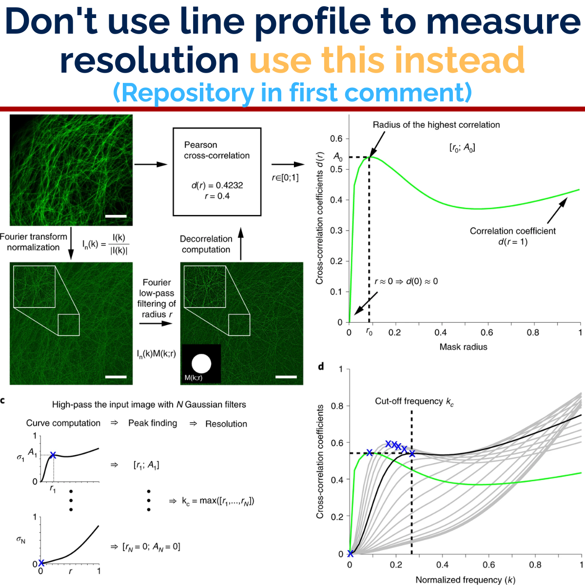
The principle rests on a clean physical distinction. Real signal and noise behave differently in Fourier space: signal is bandwidth-limited, confined below some spatial frequency set by the optics, while noise is spread across all frequencies. By cross-correlating the image with progressively high-pass filtered versions of itself, the algorithm tracks how correlation decays and identifies the frequency where meaningful signal gives way to noise.
That crossover frequency is your resolution — computed from the entire image, not from one hand-picked cross-section. The estimate reflects the data you actually collected, including the awkward regions a line profile would have skipped.
What it looks like in practice
The part that surprised me is how well it generalises. The same algorithm runs across modalities without retuning, and the implementation is genuinely easy to adopt.
What decorrelation analysis gives you
- One algorithm, many modalities confocal, STED, SIM, SMLM and brightfield all use the same method
- Precision of roughly ±1 to 3 nm tight enough to compare acquisitions meaningfully
- Signal-to-noise tracking over time useful for watching bleaching across a time series
- Open and free an ImageJ plugin plus open-source MATLAB code
The MATLAB code was straightforward to run, so I have already adapted it into part of my own image-analysis pipeline. That is a low barrier for a metric that removes so much subjectivity.
Beyond characterisation: toward self-driving microscopes
There is a longer-term reason this matters. A parameter-free, real-time resolution metric is one of the building blocks a self-driving microscope needs. If a system can continuously and honestly assess its own imaging quality — without a human drawing lines — it can adjust acquisition settings on its own, optimising for the sample in front of it rather than for a preset.
That is a different ambition from writing a cleaner methods section. It reframes resolution measurement as something an instrument does for itself, moment to moment, and decorrelation analysis is a credible candidate for that feedback signal.
One honest caveat
No method is free of failure modes. On sparse single-molecule localisation images — where there are very few localisation events — the decorrelation estimate can be optimistic. If your reconstruction is thin, treat the number with the same caution you would give any statistic drawn from too little data, and cross-check it.
That caveat aside, the shift is worth making. A line profile tells you a flattering story about one structure. Decorrelation analysis tells you what your image can actually resolve, and it does so without asking you to make the choices that bias the answer.
If you want to try it, the original paper is at doi.org/10.1038/s41592-019-0515-7 and the code is on GitHub at github.com/Ades91/ImDecorr.
So here is my question back to the community: do you still rely on line profiles, or have you moved to something more systematic? I am genuinely curious what others reach for.